

Undergraduate Open Day
Register for the SOAS Open Day and attend taster lectures, tour the Bloomsbury campus, meet our academics, and learn about our extensive range of undergraduate programmes.
Book your place